Machine Learning: Deep NeuroEvolution, Meta Learning (42)

Deep NeuroEvolution will leverage Evolution Strategies to find the best weights of the controller's linear matrix, i.e. the weights that will maximize the total reward on a full game episode. This technique is at the heart of the Policy Gradient branch of Artificial Intelligence, which therefore strengthen the hybrid nature of the Full World Model, since indeed it combines Deep Reinforcement Learning (with its use of CNN, VAE, MDN-RNN neural networks) and Policy Gradient (with its use of Evolution Strategies to find the best parameters of the controller playing the actions).

The reason why we have this image is not random, it is because evolution strategies are based, as I told you, on genetic algorithms, which consist of finding an optimal population of parameters which will lead to the best score that you define through an objective function or score function.

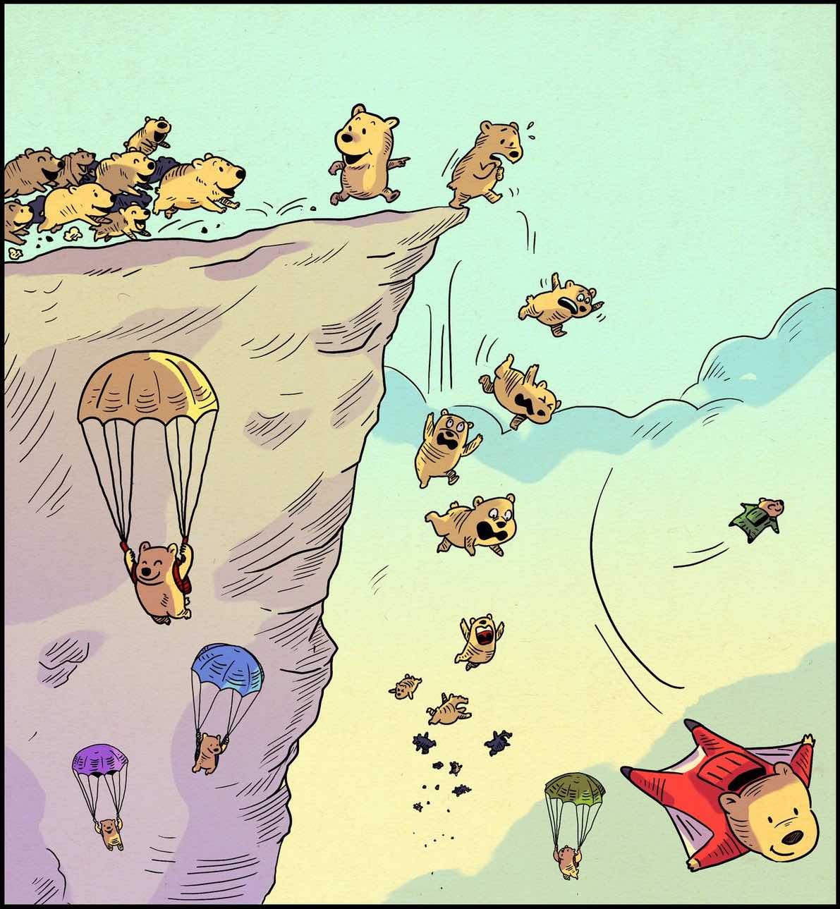
And so all the bears, little bears that you see here, are exactly the parameters, some will die, they won't be the optimal parameters, and some will survive to in the end give the best parameters.

The suit bear at the right low corner is of course the best parameters, it is the one that will stay longest in the air. So, it’s the best parameter.

Why we need Evolution strategies?

Neural network models are highly expressive and flexible, and if we are able to find a suitable set of model parameters, we can use neural nets to solve many challenging problems. Deep learning’s success largely comes from the ability to use the backpropagation algorithm to efficiently calculate the gradient of an objective function over each model parameter. With these gradients, we can efficiently search over the parameter space to find a solution that is often good enough for our neural net to accomplish difficult tasks.

However, there are many problems where the backpropagation algorithm cannot be used. For example, in reinforcement learning (RL) problems, we can also train a neural network to make decisions to perform a sequence of actions to accomplish some task in an environment. However, it is not trivial to estimate the gradient of reward signals given to the agent in the future to an action performed by the agent right now, especially if the reward is realised many timesteps in the future. Even if we are able to calculate accurate gradients, there is also the issue of being stuck in a local optimum, which exists many for RL tasks.

A whole area within RL is devoted to studying this credit-assignment problem, and great progress has been made in recent years. However, credit assignment is still difficult when the reward signals are sparse. In the real world, rewards can be sparse and noisy. Sometimes we are given just a single reward, like a bonus check at the end of the year, and depending on our employer, it may be difficult to figure out exactly why it is so low. For these problems, rather than rely on a very noisy and possibly meaningless gradient estimate of the future to our policy, we might as well just ignore any gradient information, and attempt to use black-box optimisation techniques such as genetic algorithms (GA) or ES.

OpenAI published a paper called Evolution Strategies as a Scalable Alternative to Reinforcement Learning where they showed that evolution strategies, while being less data efficient than RL, offer many benefits. The ability to abandon gradient calculation allows such algorithms to be evaluated more efficiently. It is also easy to distribute the computation for an ES algorithm to thousands of machines for parallel computation. By running the algorithm from scratch many times, they also showed that policies discovered using ES tend to be more diverse compared to policies discovered by RL algorithms.

Let’s start learning :

Do we know what this is?

This is a Rastrigin function

We use Rastrigin and Schaffer function to evaluate different optimizers

From the Rastrigin graph , we can see that it is not convex, because it has a series of mountain shapes, which therefore results in having a lot of local optima, you know local minimum and maximum. So, a classic technique like gradient descent would not be able to find the global maximum,that's why the title of this graph is two-dimensional Rastrigin function has many local optima. And so we have to use some other techniques, and these other techniques are of course evolution strategies.

Here in the Rastrigin 2d function (right one) ,

the lighter the color is, the closer we are to the maximum, and as you can see we have here some lighter points, which are neighbors to darker points, redder points, and that's how we can clearly see, even in a 2D plan, that indeed we have many local optima.

However, as you can see, the closer we get to this area here,the more lighter the color become . So, that’s the optimal goal

Make sure you understand that here, the axes are x and y, and the color, and how light it is, represents the z axis here, which is given by F(x,y). Our goal is not to find the maximum f, our goal is to find the parameters x and y that will lead to this maximum f.

Comparing this with the Full World Model’s Controller

So, in a full world model , x and y are actually Wc (W​c​​ and bc​​ are the weight matrix)

And then, this f here is exactly that score function that we have to maximize or you know,

it is that expected cumulative reward of the agent that we have to maximize.

Finally in this 3D shape of the Schaffer function, but we can clearly see that here we alternate between red circles(b) and yellow circles (a)

meaning that we clearly have those mountains here, which however becomes higher and higher mountains until we reach the highest mountain, leading us to the maximum (m), and for each of the evolution strategies technique we will see the way it is getting closer and closer to that maximum.

Simple Evolution Strategy

One of the simplest evolution strategy we can imagine will just sample a set of solutions from a Normal distribution, with a mean μμ and a fixed standard deviation σσ. In our 2D problem, μ=(μx,μy)μ=(μ​x​​,μ​y​​) and σ=(σx,σy)σ=(σ​x​​,σ​y​​). Initially, μμ is set at the origin. After the fitness results are evaluated, we set μμ to the best solution in the population, and sample the next generation of solutions around this new mean.

Using simple evolution strategy, we can reach the local maxima You can visualize that in both of the graphs

In the visualisation above, the green dot indicates the mean of the distribution at each generation, the blue dots are the sampled solutions, and the red dot is the best solution found so far by our algorithm.

This simple algorithm will generally only work for simple problems. Given its greedy nature, it throws away all but the best solution, and can be prone to be stuck at a local optimum for more complicated problems. It would be beneficial to sample the next generation from a probability distribution that represents a more diverse set of ideas, rather than just from the best solution from the current generation.

Simple Genetic Algorithm

One of the oldest black-box optimisation algorithms is the genetic algorithm. There are many variations with many degrees of sophistication, but I will illustrate the simplest version here.

The idea is quite simple: keep only 10% of the best performing solutions in the current generation, and let the rest of the population die. In the next generation, to sample a new solution is to randomly select two solutions from the survivors of the previous generation, and recombine their parameters to form a new solution. This crossover recombination process uses a coin toss to determine which parent to take each parameter from. In the case of our 2D toy function, our new solution might inherit xx or yy from either parents with 50% chance. Gaussian noise with a fixed standard deviation will also be injected into each new solution after this recombination process.

The figure above illustrates how the simple genetic algorithm works. The green dots represent members of the elite population from the previous generation, the blue dots are the offsprings to form the set of candidate solutions, and the red dot is the best solution.

Genetic algorithms help diversity by keeping track of a diverse set of candidate solutions to reproduce the next generation. However, in practice, most of the solutions in the elite surviving population tend to converge to a local optimum over time. There are more sophisticated variations of GA out there, such as CoSyNe, ESP, and NEAT, where the idea is to cluster similar solutions in the population together into different species, to maintain better diversity over time.

Learn the whole theory from here

Covariance-Matrix Adaptation Evolution Strategy (CMA-ES)

A shortcoming of both the Simple ES and Simple GA is that our standard deviation noise parameter is fixed. There are times when we want to explore more and increase the standard deviation of our search space, and there are times when we are confident we are close to a good optima and just want to fine tune the solution. We basically want our search process to behave like this:

Amazing isn’it it?

In our first evolution strategy (Genetic Algorithms), the simple evolution strategy. Remember that the standard deviation, sigma, was fixed, and that's why that the blue points surrounding the green point are always in the same range, well, you know that's the simple points, always in the same circle around the mean. Well, that's because the standard deviation was fixed but now the particularity of the CMA-ES Evolution Strategy is that it is no longer fixed, the standard deviation noise parameter is no longer fixed, and that's why that now you see some blue points surrounding the mean within different ranges.And that's a much better solution because indeed, if you have different mountain shapes like, you know, not necessarily higher and higher. Well, you might get stuck in your local optima, you might not be able to reach the global maximum if, indeed, the standard deviation is fixed. But now, because the standard deviation is varying over time, over the iterations. Well, when the standard deviation is large enough, well, you will be able to go over a higher mountain in that series of mountain shapes to, therefore, be able to catch that global maximum. So, it is by far one of the best evolution strategies with, the other one, which is the PEPG, we'll come to that later.

Remember that CMA-ES is used for a reasonable amount of parameters, meaning less than 1000. But when you have thousands of parameters to optimize, you will rather use PEPG*.*

But in our case the full world model where, you know, the controller is simply a single layer linear model. Well, we definitely don't have thousands of parameters and therefore, the CMA-ES is clearly the best evolution strategy to use for that particular case.

Learn more from here

Natural Evolution Strategies/Parameter Exploring Policy Gradients (PEPG)

Before we had either the simple evolution strategy where we simply sampled a set of parameter solutions from a normal distribution of a fixed standard deviation sigma, and then we covered the covariance-matrix adaptation evolution strategy, where same, we sampled a set of parameter solution, but this time with a varying standard deviation sigma, or more specifically a varying covariance-matrix C, with that adapted computation of the covariance by taking the mean of the previous generation, and each time, well the idea is that we sampled a set of parameter solution from that normal distribution, and inside the set of sampled solutions, well, we took the best solution, the red point, and we updated the mean according to that best solutions.

And besides, in that last evolution strategy we've covered, the CMA-ES, well remember that we actually took the 25% best solutions to compute that adapted covariance matrix. And so, here we're gonna see a couple of things to change.

The first one is that this time instead of taking a sub-set of best solutions to only keep the best solutions, well, we're gonna keep this time even the worst solutions. And that is because, as author clearly states, weak solutions contain information about what not to do. That's the classic learn from the mistakes. Well, the weak solutions, the worst solutions, will tell the evolution strategy what direction to avoid in order to find that optimal set of parameters. So that's the first thing that change. We're not gonna take, for example as before, 25% of the best solutions to sample the next generation. But then the second thing that change, and which is pretty big, is that this time we're gonna use again the classic gradient to update the parameters.

The center of the natural evolution strategies is exactly what we see here. The parameter update through the gradient.

θ→θ+α∇​θ​​J(θ)

This right here, nabla of J theta, is the gradient of J theta, where J is an objective function. So you have to know about objective functions.

Learn more here

Open AI Evolution Strategy

In OpenAI’s paper, they implement an evolution strategy that is a special case of the REINFORCE-ES algorithm outlined earlier. In particular, σσ is fixed to a constant number, and only the μμ parameter is updated at each generation. Below is how this strategy looks like, with a constant σσ parameter:

In addition to the simplification, this paper also proposed a modification of the update rule that is suitable for parallel computation across different worker machines. In their update rule, a large grid of random numbers have been pre-computed using a fixed seed. By doing this, each worker can reproduce the parameters of every other worker over time, and each worker needs only to communicate a single number, the final fitness result, to all of the other workers. This is important if we want to scale evolution strategies to thousands or even a million workers located on different machines, since while it may not be feasible to transmit an entire solution vector a million times at each generation update, it may be feasible to transmit only the final fitness results. In the paper, they showed that by using 1440 workers on Amazon EC2 they were able to solve the Mujoco Humanoid walking task in ~ 10 minutes.

I think in principle, this parallel update rule should work with the original algorithm where they can also adapt σσ, but perhaps in practice, they wanted to keep the number of moving parts to a minimum for large-scale parallel computing experiments. This inspiring paper also discussed many other practical aspects of deploying ES for RL-style tasks, and I highly recommend going through it to learn more.