Until now, we had data which we could separate with a line.

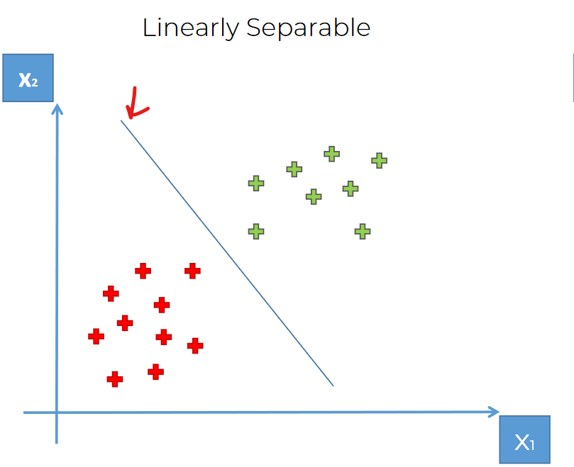
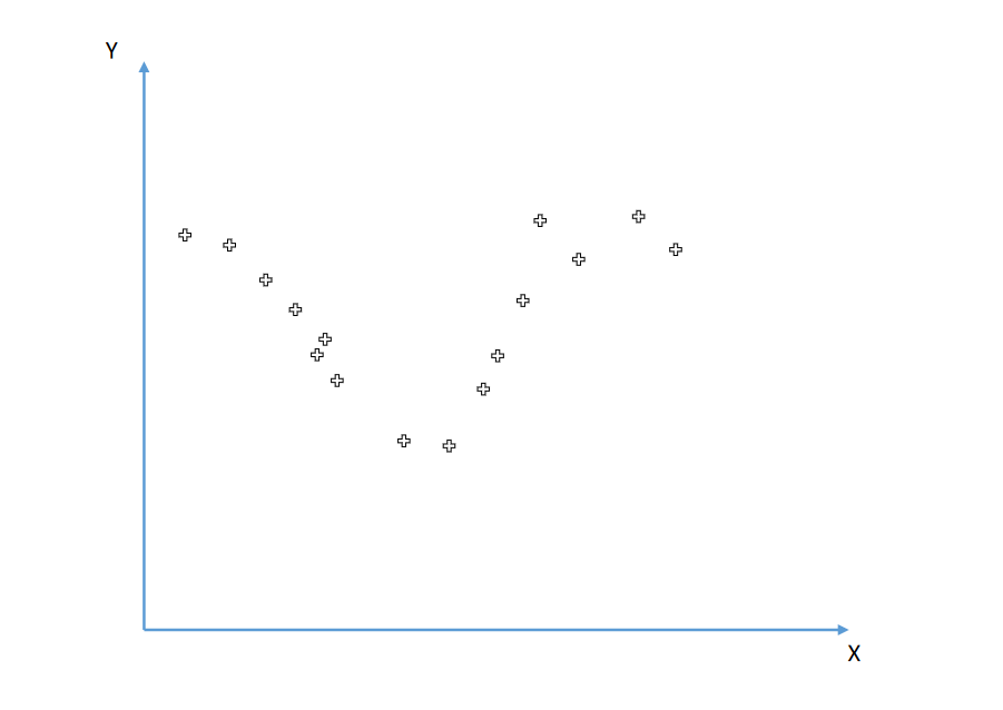
But what if we get data like this?

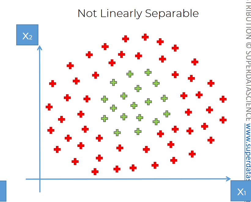
Now we can't use any linear lines to separate them.

There are few ways to separate them.Ways:

1. We can go to higher dimension:

   

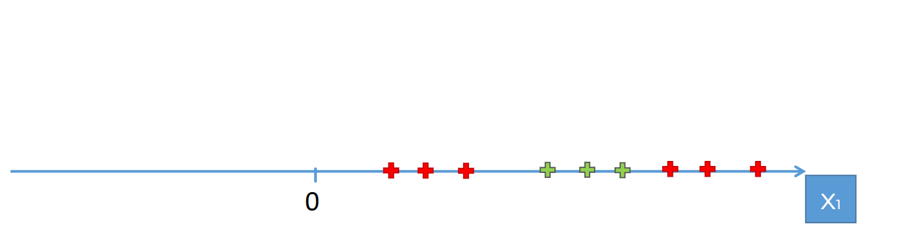
   Assume that we have some data on this line (1D). We can not simply separate them with 1 dot. We will need two at least.

   

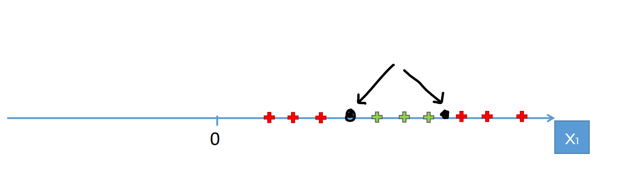
   But what if we take x=5 where y=0

   

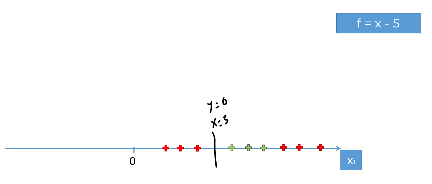
   We can now see those red crosses to shift to left. and set y=0 at x=6

   Then f=(x-5)^2

   

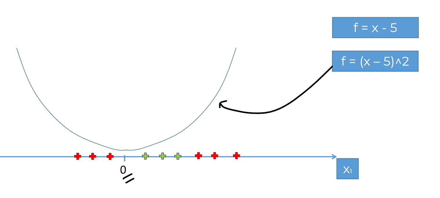
   This gives us a Parabola.

   Now, if we fit all of our data to this parabola, we can create a line . Let's see:

   

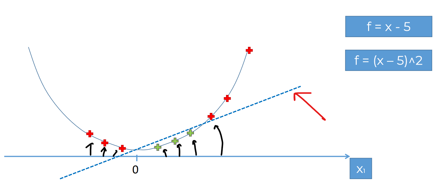
   You can see how we took our 1D line to a 2D line and then managed to have a line to separate them

   Remember, in 1D plane , we need 1 dot, in 2D plane, we need a line and in 3D plane, we need a hyperplane to separate data

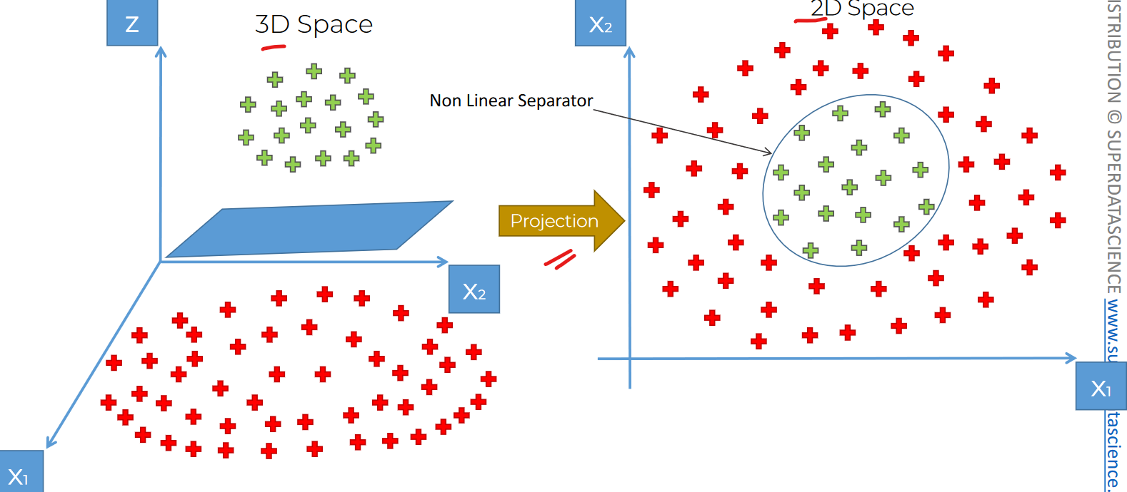
   In the same way, we can take this 2D data to 3D and manage a plane to separate them.

   

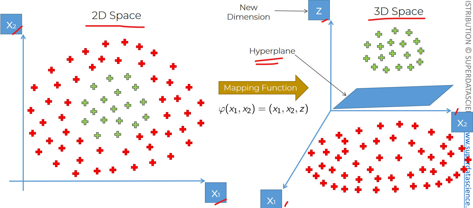
   We would need a Mapping function for that.

   Again, from 3D to 2D, we can use projection to do this.

   

   Issues:

   • Mapping to higher dimension is very highly compute impulsive. So, we will need a high end processor etc.

2. Kernel trick:

   

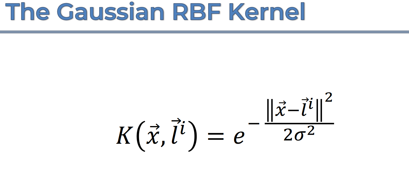
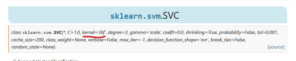
   This is Gaussian RBF kernel. Note that, we did see kernel='rbf' in our sklearn documentation for SVM

   

   

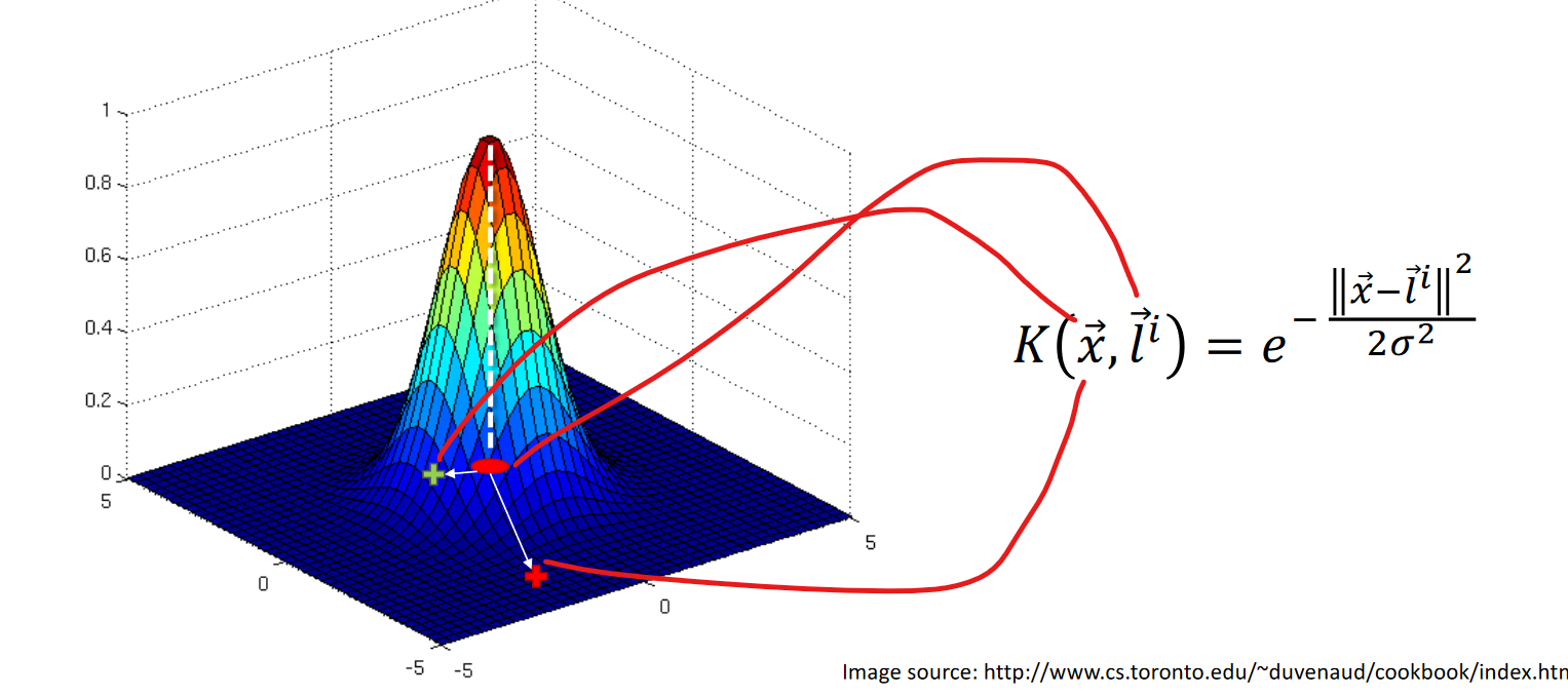
   Here dot red is the landmark(l) and from x, we can check out the distance.

   So, in 2D plane, we can use this Gaussian kernel

   

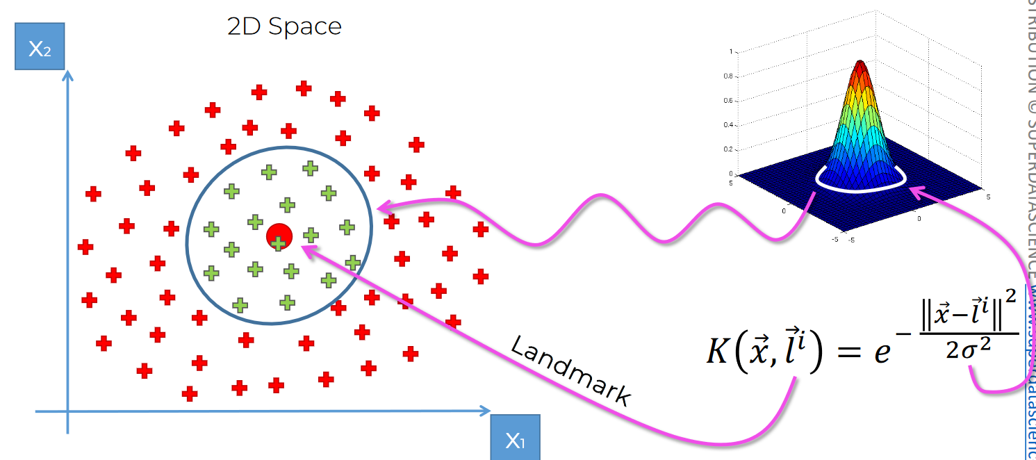
   here, red dot is Landmark and sigma defines the circumference

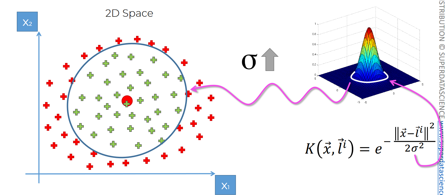
   If sigma increases, the circumference increases.

   

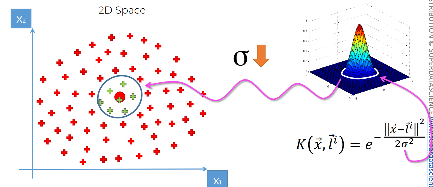
   Same goes when it decreases

   

   Again for data like this, we can use 2 Gaussian kernel

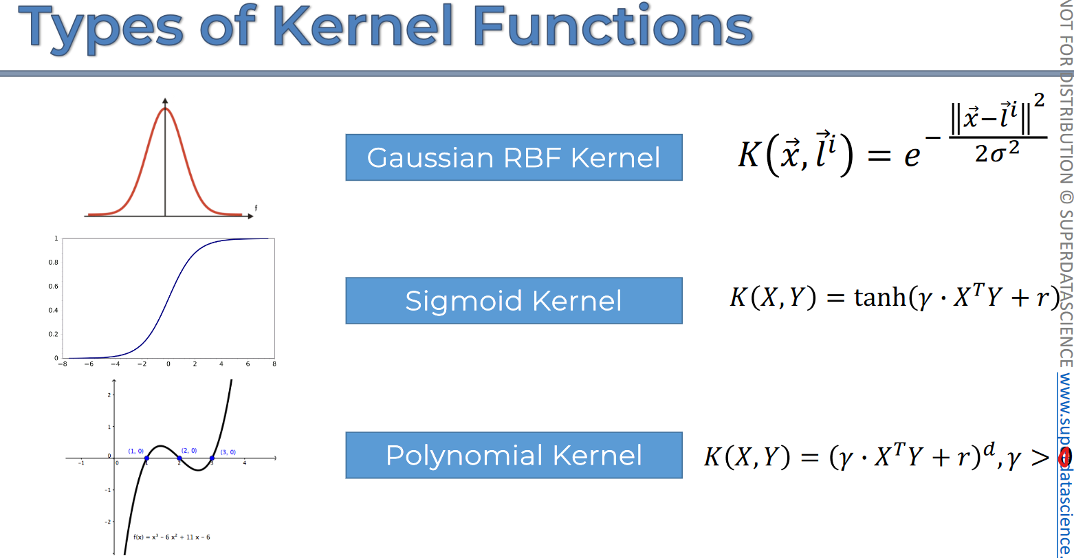
   Types of kernel functions:

Types of Kernel functions

Non Linear SVR

Assume we have data in this 2D plane

We can't separate them with a line

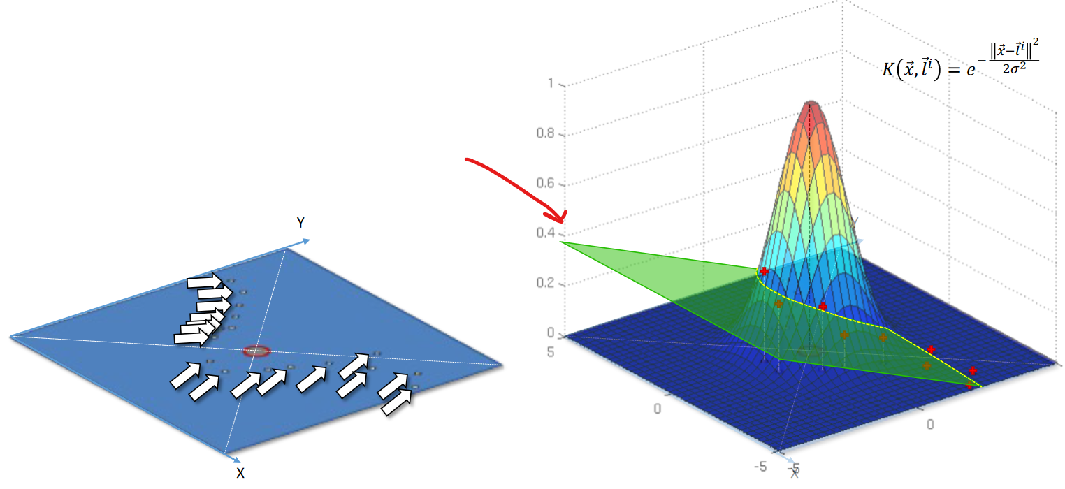
Let's create a box with this 2D plane and keep it on the ground like this.

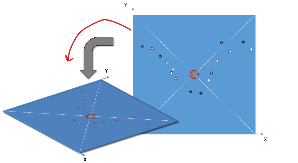
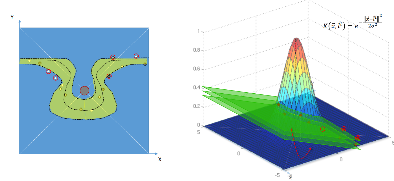
Now if we use Kernel rbf, we can see

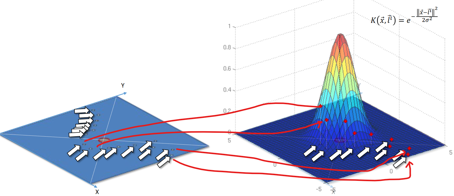
All of the data plotted in 2D can bee seen in the 3D plot on right.Now in the 3D , we can use hyperplane to separate the data

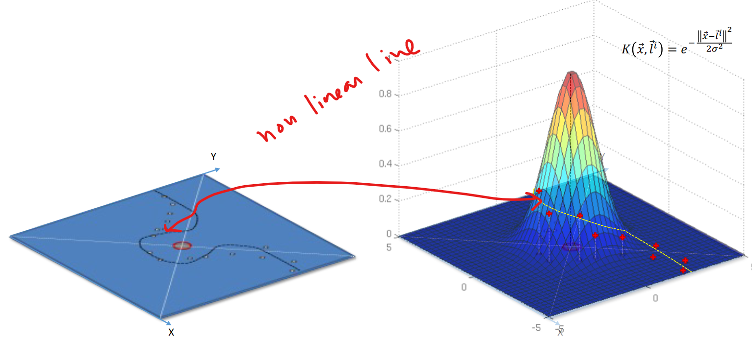
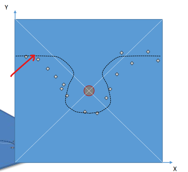
This creates a non-linear line on the plane. If we try to see it's projection on the 2D plane . We can see like this.

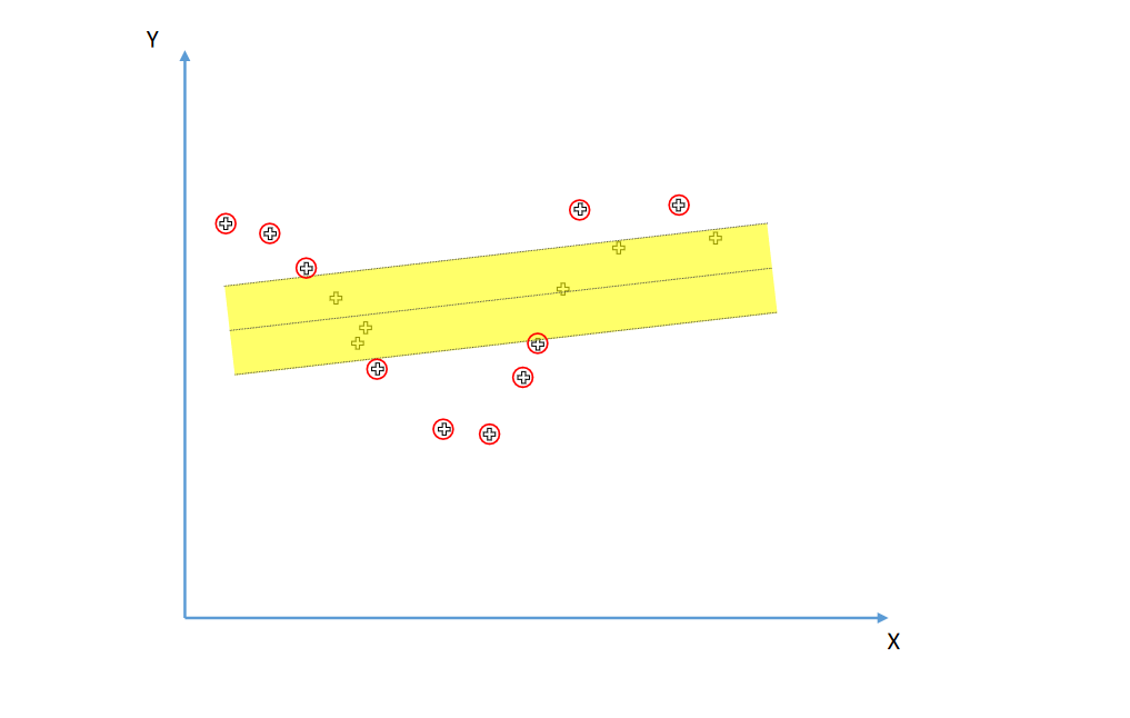
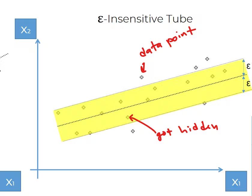
You may ask, why are we still calling Support Vector Regression?

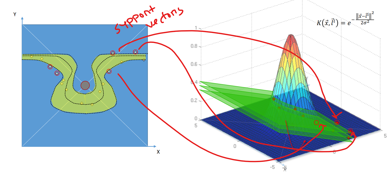
if we basically create 2 more plane, we can see 1 epsilon tube to be created . And we can see some supported vectors which is supporting the tube. Isn't this how we got the idea of support vector?

This image is shared to make you remind about our epsilon tube concept for Support vector

So, That's it.

We have successfully created a SVR

Let's code it down

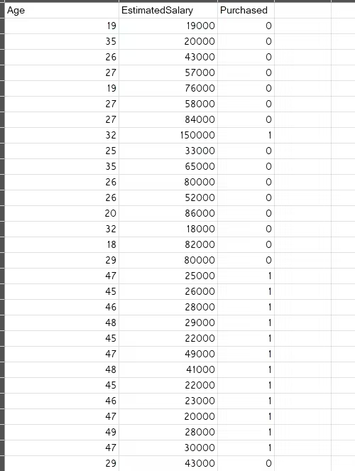
Problem statement: We are launching a new SUV in the market and we want to know which age people will buy it. Here is a list of people with their age and salary. Also, we have previous data of either they did buy any SUV before or not.

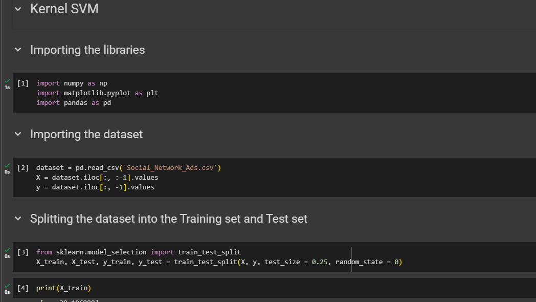
So, import libraries , dataset and split the data

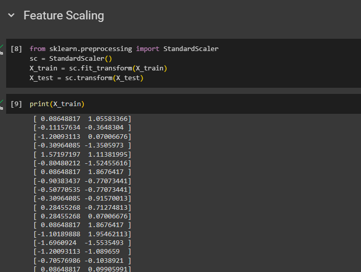
Feature scale the X matrix data

Training the Kernel SVM model on the Training set

from sklearn.svm import SVC

classifier = SVC(kernel = 'rbf', random_state = 0)

We have multiple options for the kernel and we are using setting the kernel to 'rbf'

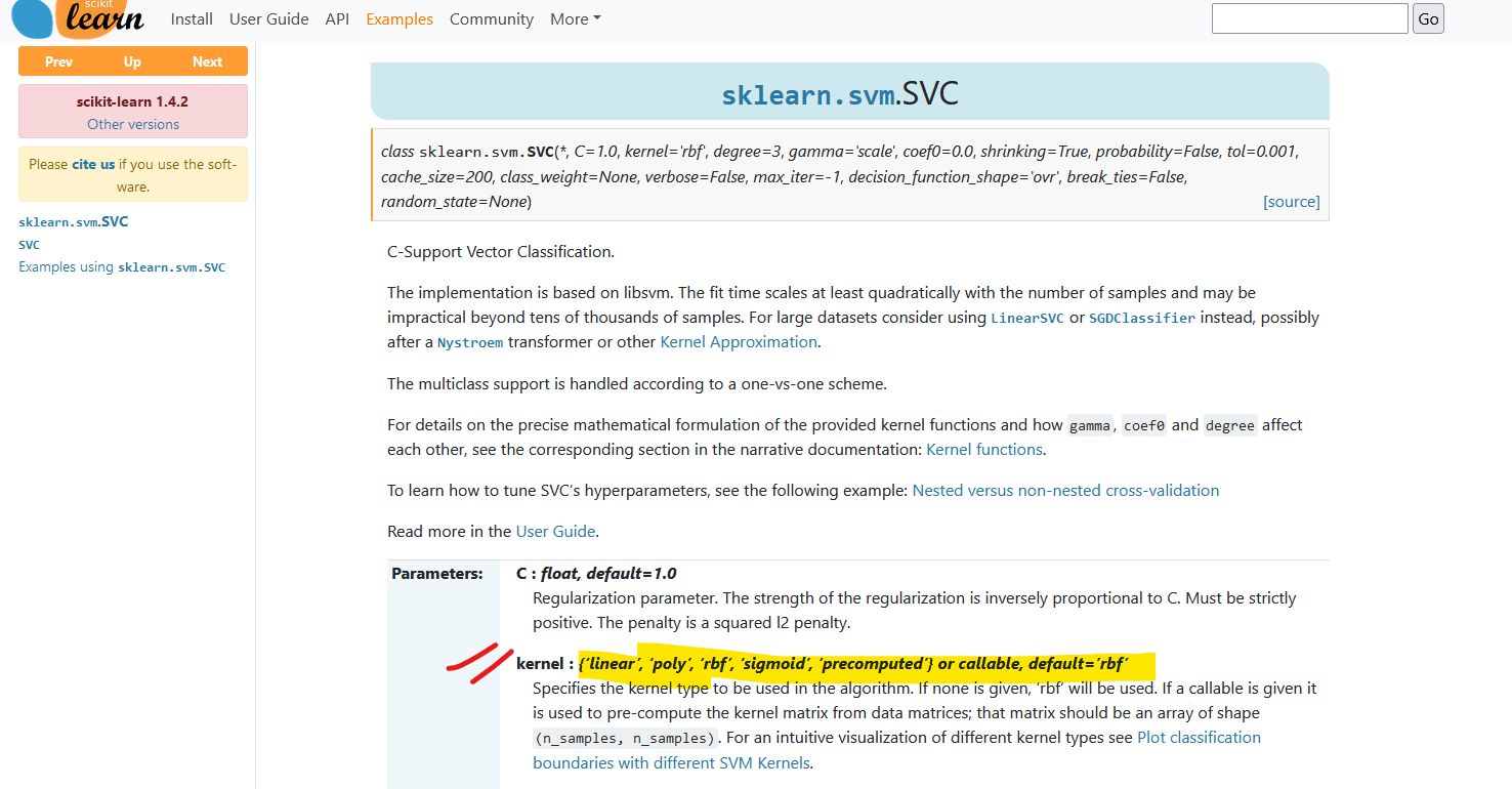
Check out the documentation

classifier.fit(X_train, y_train)

Predicting a new result

Predicting for a 30 year person with salary 87000

print(classifier.predict(sc.transform([[30,87000]])))

Predicting the Test set results

y_pred = classifier.predict(X_test)

print(np.concatenate((y_pred.reshape(len(y_pred),1), y_test.reshape(len(y_test),1)),1))

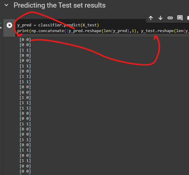
Now we can see our prediction and our test data side by side

Making the Confusion Matrix & accuracy

from sklearn.metrics import confusion_matrix, accuracy_score

cm = confusion_matrix(y_test, y_pred)

print(cm)

accuracy_score(y_test, y_pred)

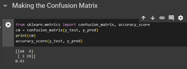
We can see 93% accuracy here.

Visualizing the Training set results

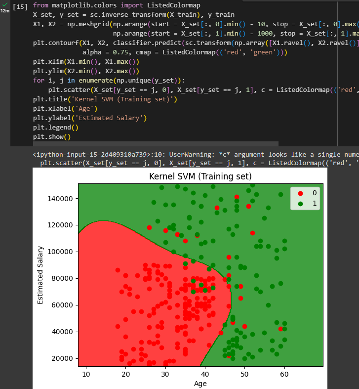
You can see non-linear lines to separate the data well.

Visualizing the Test set results

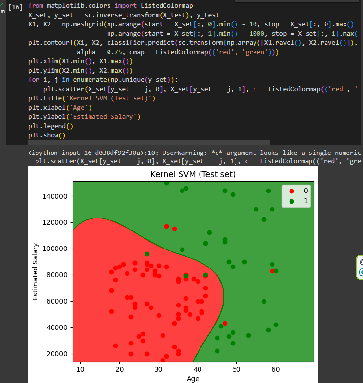
Done!

Here is the code

Here is the dataset

Thank you